| Tests can be run for either tracking method using either
one or three "balls". Noise can be injected into the generation
of the data but is scaled according to the parameter. The injection
process occurs in two passes to mimic the two kinds of noise, model and
measurement, that exist in a tracking system. Two kinds of unimodal
noise are used to perturb the data: Gaussian and Triangular. Finally, for
the three-ball scenario, the synthesized "measurements" are
randomly re-ordered within a given measurement timestamp.
Bouncing Ball Model
Time-based parametric equations were used to model the bouncing balls.
Horizontal velocity was kept constant with the exception of applied
constant drag (as a multiple, not a subtraction to make the Kalman 'A'
matrix easier to program later). Vertical velocity was affected by
constant acceleration and drag. The same acceleration was used for all
balls (simulating the idea that gravity at one location affects everything
in pretty much the same way). For ease of calculation, the "scale
argument" was used to justify using "1" as dt.
Consequentially, the equations (ignoring 'k' and 'k-1' subscripts) look
like:
x = x + Vx
(the expected " * dt" is eliminated because of the dt
= 1 definition)
y = y + Vy
Vx = Vx * drag
Vy = Vy * drag + Ay
Ay = Ay
Where
x := measurement in x dimension
y := measurement in y dimension
Vx := velocity in x dimension
Vy := velocity in y dimension
Ay := acceleration in y dimension
The three balls are initialized in different locations and in started
in different directions. Two bounce from left to right, one bounces from
right to left.
Unimodal Distributions
Two different unimodal distributions were used to draw samples from: a
normal, or Gaussian distribution as implemented in OpenCV and a
"Triangular" distribution. In both cases, the results were
scaled and shifted to return values between -1 and 1 to make application
via on a noise factor easier.
Model Noise
In the first pass, noise is injected into the model parameters Vx, Vy,
and Ay. The noise factor is multiplied by one of the unimodal
distributions and subsequently scaled to simulate the idea that some model
parameters are more likely to be affected than others and that, hopefully,
the model noise is much 'quieter' than the measurement noise. Hence, the
velocity parameters are scaled by 0.1 and the acceleration parameter by
0.01.
Measurement Noise
In the second pass, noise is injected into the X and Y coordinates of the
data generated in the first pass. Again, noise is drawn from one of the
unimodal distributions and multiplied (without further scaling) by the
supplied noise factor.
|
At the highest level, tracking with Kalman filters involves
initializing the OpenCV CvKalman structure and
following the sequence:
- Predict (calling cvKalmanPredict)
- Associate with a measurement (using a proprietary algorithm)
- Correct using the measurement (calling cvKalmanCorrect)
Initialization
Initialization consists of constructing a model transition matrix A,
the process noise covariance matrix Q, the measurement covariance matrix
R, the measurement transition matrix H found in the formulas:
x(k) = Ax(k-1) + w(k-1)
z(k) = Hy(k) + v(k)
where x is a model vector, z is a
measurement vector, w is model noise drawn from the
distribution identified by Q and v is the
measurement noise drawn from the distribution identified by R.
In our case, all the parameters are independent and we pretend there is
no transformation needed to convert measurement vector data into model
vector data (e.g. rotation or scaling). Therefore, the H matrix is
initialized as an identity matrix, the R matrix is initialized as a
one-valued diagonal with the value specified by the experiment, and the Q
matrix is also initialized as a one-valued diagonal again with the value
specified per experiment. Had there been any dependencies (say, between
the velocities, we would have needed to encode those in the covariance
matrices.
The A matrix is tightly coupled with our state vector and represents
our expected transformation of a given state. In other words, it tells us
how the parameters change with each iteration or time step. In algebraic
form, using all parameters, it looks like:
1*x + 0*y + 1*Vx + 0*Vy + 0*Ay = x
0*x + 1*y + 0*Vx + 1*Vy + 0*Ay = y
0*x + 0*y + 1*Vx + 0*Vy + 0*Ay = Vx
0*x + 0*y + 0*Vx + 1*Vy + 1*Ay = Vy
0*x + 0*y + 0*Vx + 0*Vy +10*Ay = y
It's easy then to see that the matrix for A should be:
| 1 |
0 |
1 |
0 |
0 |
| 0 |
1 |
0 |
1 |
0 |
| 0 |
0 |
1 |
0 |
0 |
| 0 |
0 |
0 |
1 |
1 |
| 0 |
0 |
0 |
0 |
1 |
We make one change to represent the drag on the velocity and replace 1
with a drag constant (less than 1):
| 1 |
0 |
1 |
0 |
0 |
| 0 |
1 |
0 |
1 |
0 |
| 0 |
0 |
Drag |
0 |
0 |
| 0 |
0 |
0 |
Drag |
1 |
| 0 |
0 |
0 |
0 |
1 |
The initial state is calculated by first associating each of the three
Kalman structures with each of the first three points (we don't care
which). Next, we use a simple "closest" algorithm to match the
first set of three measurements with the next set of three measurements
(since we don't know which measurement belongs to which ball having
randomized it). From this pairing, we can make an estimate of the
velocities (Vx = x1 - x2, etc.) and we set Ay to a "known"
constant.
Data Association
At each step, we need to associate the Kalman tracking structure with a
measurement from a set of observations. The chosen (and only partially
successful) algorithm was what could be called
closest-in-the-right-direction. We evaluate the three measurements, pick
the one(s) that are closest to our current position and, if there are more
than one, pick the closest one that's in the quadrant we're moving
towards.
Results
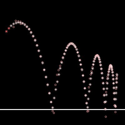
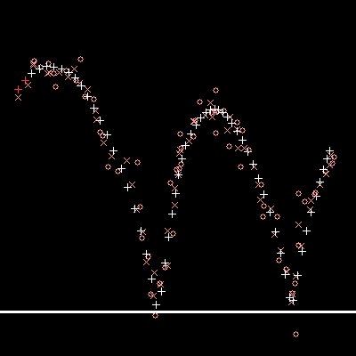
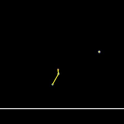
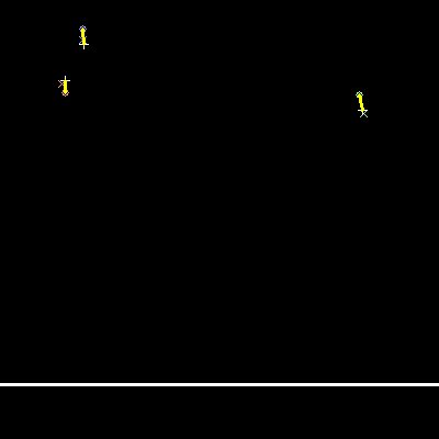
In the movies that follow, white crosses represent the actual data,
colored X's represent a measurement, and circles represent the Kalman
filter's estimate of where the ball is.
| Description |
Movie |
| Kalman filter tracking of a single ball with no noise
injected. Notice the estimate overshoots the "floor" and
then overcompensates before settling down. |
 |
| Kalman filter tracking a single ball with a noise
factor of 10 applied. |
 |
| Kalman filter tracking three balls (cumulative
recording turned off, lines showing distance between estimate and
actual data turned on) with no noise. Notice how two filters end up
getting associated with one set of measurements leaving another set
abandoned. |
 |
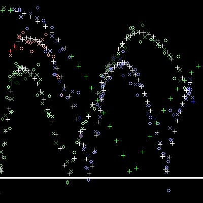
| Kalman filter tracking three balls with a noise factor
of 5 with estimate/data differences emphasized. |
 |
| Kalman filter tracking three balls with a noise factor
of 10 with cumulative display turned on. Notice that a different
ball gets orphaned. |
 |
 |
Graph of the errors of the above experiment. |
|
| Particle filters work kind of like the Yatzee game. To play
Yatzee, you throw the die and keep the ones that will maximize your
expectation and re-throw the remaining one in hopes of getting better
results. In the case of particle filters, you re-throw all the proverbial
die but the philosophy is similar: based on what you see, adjust things to
get better results next time.
For particle filters, samples are randomly distributed around a model,
evaluated against a measurement, the model is changed, and the process is
repeated. This is similar to the predict/correct cycle of the Kalman
filter but has a couple of twists. One twist is that you can refine your
model several times with each measurement. Another twist (which helps with
non-linear problems) is that the model is not modified merely with a
linear process; complex functions can be used to drive convergence to a
model. At a high level again, the process looks like:
- Throw out random samples around current best guess possibly using a
linear model to help
- Evaluate the samples against a measurement (using complex functions
if desired)
- Rinse and repeat.
Or, to quote Maskell and Gordon [2001], "the key idea is to
represent the posterior density function by a set of random samples with
associated weights and to computer estimates based on these samples and
weights."
Initially, I had intended to use the same transition matrix (A) from
the Kalman filter exercise in the "throw out random samples"
phase. I quickly realized that this would impose a problem on hoping to
re-apply condensation several times for a given measurement. Let's take a
simple example: suppose I presume that the thing I'm tracking moves to the
right about 6 units every measurement. If I incorporate that model into
the condensation tracking, then each time I throw out the samples I move
them 6 units to the right (plus the noise). If I try to apply condensation
three times for every measurement, then I'm moving the thing 18 units to
the right! I was reminded of the fact that the transformation is linear
and hence I can scale it down based on the expected applications [Boult
2004]. Thus, if I want to model something that moves 6 units and am going
to apply the transformation 3 times, I simply move it 2 units in each
transformation. In linear terms, f(ax) = af(x).
However, it was too late to apply this knowledge so I just followed the
simplest of all models: presume nothing happens and then modify the
probabilities against the actual measurement. The question then becomes
how much of an efficiency gain could I obtain by incorporating the model.
Could I reduce the number of iterations from five to, say, three and still
get the same accuracy?
Assigning Probability
The most important feature, at least when using OpenCV, for using particle
condensation filters is the evaluation function. We need to assign
probability weights to each sample based on the latest measurement so that
the cvConDensUpdateByTime function can resample properly. Ideally, in the
case of the bouncing balls, I could assume a Gaussian distribution around
the mean (best guess of the ball's x/y position). Simpler still, we can
just measure the distance from each sample and weight this in a Gaussian
manner. Good ideas, but they didn't seem to work well (the samples never
swarmed to the data). So in desperation, I tried the simplest of all
models: an inverse function of the distance (no Gaussian weighting). It
worked beautifully. So even with the simplest of models, the process was
quite convincing.
Data Association
A much more successful data association strategy was employed after seeing
the one used with the Kalman filter yield less than desirable performance.
In this case, we take each condensation model and search among the
measurements for the closest one. Once we find it, we associate the
condensation structure with it and then remove the measurement from
further consideration. This is the "middle-school dance partner"
strategy with an equal number of "guys" and "gals". We
don't actually care if a condensation structure switches "balls"
because another structure will pick up the orphaned ball later.
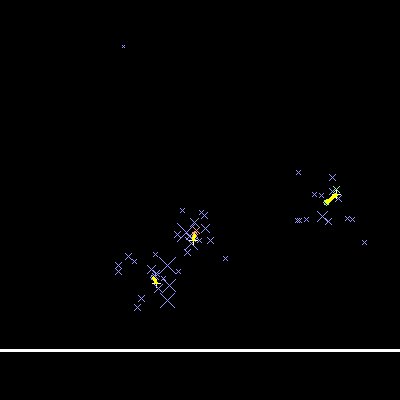
Results
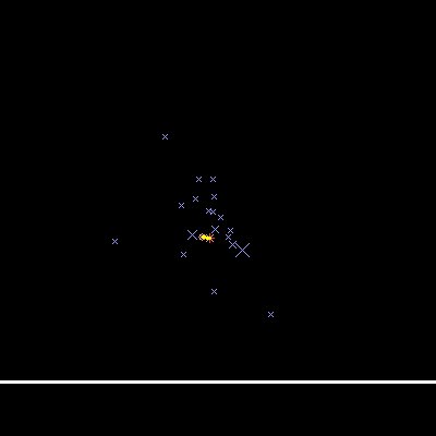
In the movies that follow, the blue X's represent the samples and,
following Dr. Boult's example, are sized to illustrate the confidence in
the sample. The white cross represents the data and colored circles
represent estimated positions and colored X's represent the measurement
data.
We actually have several more parameters at our disposal so our
possible combination of results is quite large. Only a few representative
examples are shown.
| Description |
Movie |
| One ball with no noise, 20 particles, only one
condensation per measurement, an upper bound of 200 (pixels). This
means the samples can be widely thrown but then only have one chance
to converge on the measurement data. It doesn't track very well.
Nevertheless, it does avoid overshooting and overcorrecting (all
of these movies show Condensation avoids that). |
 |
| One ball with no noise, 20 particles, five
condensations per measurement, an upper bound of 200. Tracking is
much better now! |
 |
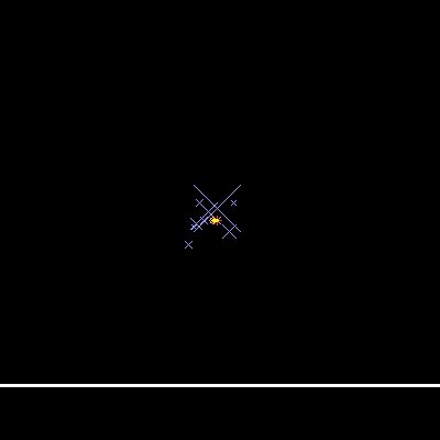
| One ball with no noise, 20 particles, five
condensations per measurement, an upper bound of 100. Samples are
not thrown as far away from the mean so we could expect better
convergence. Notice how much more tightly the ball is tracked. |
 |
| One ball with no noise, only 10 particles this time,
five condensations, an upper bound of 100. Not quite as good as 20
particles, but better than 20 particles with only one condensation
and an upper bound of 200. |
 |
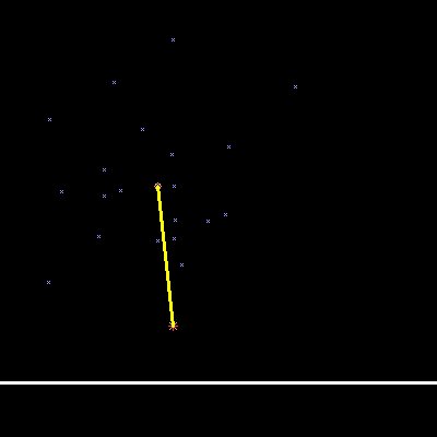
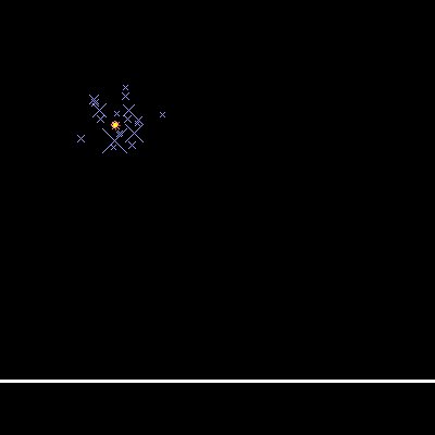
| Three balls, with no noise, 15 particles, four
condensations, an upper bound of 100. Notice that no balls get
orphaned. An interesting artifact that seems to be how the
OpenCV software initially seeds the samples is that it appears to
ignore the model's initial position. It just starts all samples
clustered near the upper left. Hence, the ball on the right has a
large deviation and takes a few iterations to correct itself. |
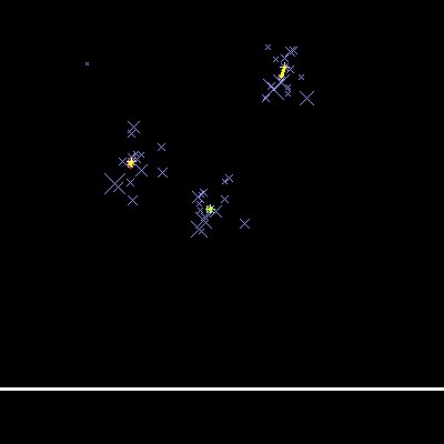 |
| Three balls, with a noise factor of 10, 15 particles,
four condensations, an upper bound of 100. |
 |
 |
Condensation Tracking errors. Note the heavy spike up
front that quickly converges for the ball on the right. |
 |
Segment from the same chart without the extremal data. |
|