Tracking Satellite-like Things Using Kalman Filters and Condensation

Tracy Petrie
University of Colorado, Colorado Springs

1. Introduction

In the previous project, we looked at a system (bouncing balls) that used position, velocity, and constant acceleration parameters. The model of the system that used these parameters was linear which made Kalman filters an especially attractive solution being relatively efficient and linear by nature. In this project, we mix it up a bit by introducing coupled components that have non-linear motion. One of the questions that is interesting (and the one focused on here) is whether simplified linear Kalman models can adequately track non-linear systems.

2. Data Generation

The objects tracked in this project were point masses (rather than real masses with 2D shape that needed to be tracked) coupled by a rigid rod. These objects were then rotated and translated in a frictionless 2D space. Data was generated by randomly creating two radii lengths (to simulate the effect of an off-center centroid caused by varying values of the two masses), an initial rotation angle, an angle velocity, and a translation vector for each object to track. The object was then rotated and moved (translated) and the point-mass locations were recorded as the event.

Unimodal Distributions
Only one Gaussian distribution was used to introduce model/measurement noise.

Model Noise
In the first pass, noise is injected into the model parameters (radii, translation velocities Vx,Vy, and angle velocity).

Measurement Noise
In the second pass, noise is injected into the X and Y coordinates of the data generated in the first pass. Again, noise is drawn from the unimodal distributions and multiplied (without further scaling) by the supplied noise factor.
 

3. Tracking with Kalman Filters

One thing that I did was to separate out the point masses and to have one Kalman filter track one point mass. In retrospect, it would have been better to work harder at associating data so that we could have tracked the dual-mass objects, not the individual masses..

Initialization
Three different models were used with Kalman filters in an effort to see how increased model complexity affected accuracy and performance. These are called in the results section below "None", "Partial", and "All". 

The "None" filter simply initializes the A matrix to the Identity matrix. In essence, this model presumes nothing changes. In fact, the only thing we pay attention to is the location of the point mass we're tracking. So the state vector is simply (x,y) and the A matrix is simply:

The "Partial" filter recognizes that constant velocity is relatively easy to model and so the velocity parameters are included. The state vector is (x,y,Vx,Vy) and the A matrix is:

The "All" filter acknowledges the fact that the sinusoidal motion (in each dimension) can be modeled with changing velocity even if the linear Kalman model cannot predict it exactly. It can (if the angular velocity is small enough) hypothetically adjust the state using the correction function to track better than the Partial filter. The state vector is (x,y,Vx,Vy,Ax,Ay,Jx,Jjy) where V is velocity, A is acceleration, and J is "jerk" (using Dr. Boult's terminology) the rate of change for acceleration. The A matrix is a bit larger this time. The initial state matrix set the acceleration values to 1 and the jerk values to 0.1.

1	0	1	0	0	0
0	1	0	1	0	0
0	0	1	0	1	0
0	0	0	1	0	1
0	0	0	0	1	0
0	0	0	0	0	1

Data Association
Due to time considerations, I simply used a "closest" algorithm. In mutliple-object tracking experiments, many point-masses were orphaned.

Experiments
To test the variations, a quadrant of four combinations of rotation/translation was created and each type of filter was tested with each quadrant's values. The idea was to contrast how well the Kalman filter tracked the objects when the major motion influence came from the rotational component relative to the translation component and visa versa. To set these measurements in perspective, we needed to also see how well it was tracking when there was very little motion and when there was a great deal of motion in each estimate/correct iteration. These values were chosen "instinctively" but a better mathematical basis probably should have been used to pick them. Also, more experimentation with the rotational velocity would tell us if there is a "sweet spot" in between the .1 and .7 values used (i.e. a curve with a local maximum). The quadrant looks like:

Results
The results are shown visually and described quantitatively. The quantitative results were obtained by tracking the distances between the estimated position and the actual (model) position with no model noise and a measurement error factor of 5 and calling this distance the error. Average and standard deviation values were obtained from only one run in each quadrant for each model type (with at least 39 values). A better experiment would probably include several runs (how many is enough?). 

The only unusual standard deviation was observed in the Q12 quadrant using the full model. This is explained by some initial tracking difficulty on the first few measurements but the subsequent error rate settled down after that and the standard deviation returned to an expected value. Interesting cases occurred in the Q11 and Q12 quadrants. In the Q11 quadrant, the partial model appeared to work best although both the partial and full models were better than the simple model. In the Q12 quadrant, the full model appeared to be dramatically better than the other models but the partial model actually got worse than the simple model. This was especially surprising because my expectation was that it would perform significantly better. I would actually expect to run this test a few more times before drawing any conclusions.

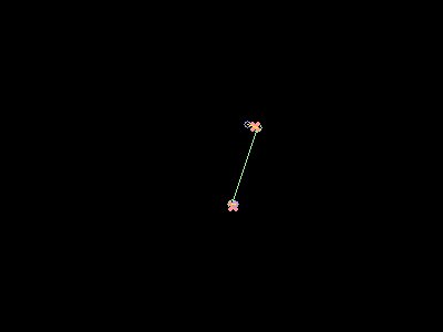
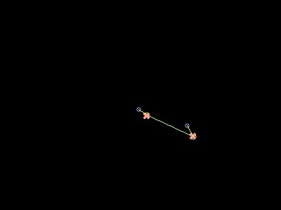
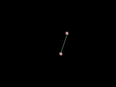
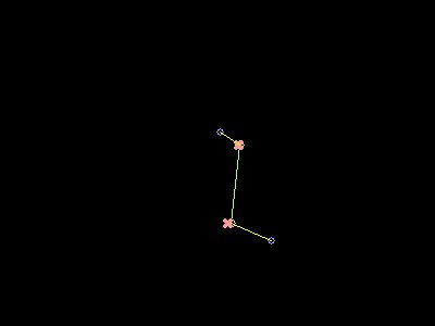
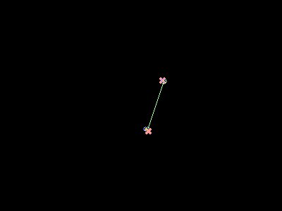
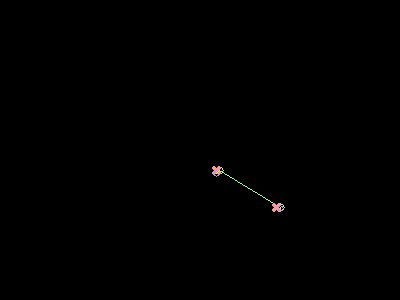
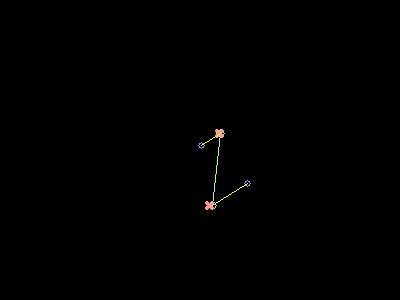
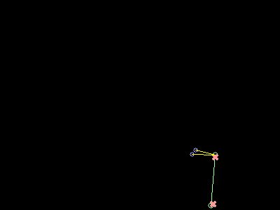
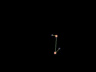
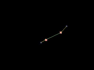
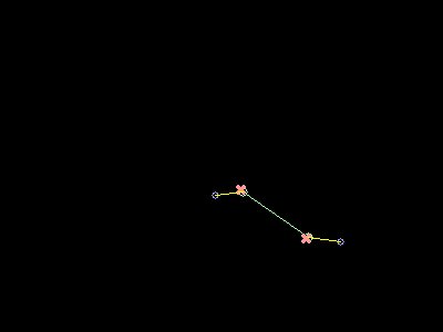
In the images, the green circles represent the point-masses (connected by the green line), the red Xs represent the measurements, and the small blue circles represent the estimated position. A yellow line connects the estimated position with the actual.

Q11 - Rotation .1, Translation 1	Q12 - Rotation .1, Translation 10
Simple model (only position used). Average Error: 6.02 Standard Deviation: 1.91	Simple model (only position used). Average Error: 18.06 Standard Deviation: 4.45
Partial model (position and constant velocity used). Average Error: 3.21 Standard Deviation: 1.41	Partial model (position and constant velocity used). Average Error: 28.61 Standard Deviation: 9.85
Full model (position, changing velocity, and changing acceleration). Average Error: 4.28 Standard Deviation: 2.15	Full model (position, changing velocity, and changing acceleration). Average Error: 5.81 Standard Deviation: 3.67
Q21 - Rotation .7, Translation 1	Q22 - Rotation .7, Translation 10
Simple model (only position used). Average Error: 32.12 Standard Deviation: 9.71	Simple model (only position used). Average Error: 29.32 Standard Deviation: 13.70
Partial model (position and constant velocity used). Average Error: 29.46 Standard Deviation: 9.53	Partial model (position and constant velocity used). Average Error: 28.91 Standard Deviation: 9.89
Full model (position, changing velocity, and changing acceleration). Average Error: 27.84 Standard Deviation: 9.40	Full model (position, changing velocity, and changing acceleration). Average Error: 27.00 Standard Deviation: 9.97

An Excel file with the data can be found here.

Other interesting movies or experiments are shown below:

Description	Movie
Tracking four objects using Kalman filter (the partial model). Compare the errors (seen by the yellow lines) with the condensation tracking below. Also note the transfer of a Kalman tracker from the lower left object to the upper left object.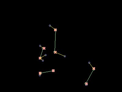
Condensation tracking of four objects. Note the absence of visible yellow lines; tracking is visually much better as would be expected given the non-linear nature of the motion.

5. Problems/Work to be Done

In addition to getting the data association model to be more accurate, we need to be able to measure the association so we can quantitatively evaluate the accuracy. 

Finally, an unmet goal of this particular project was to apply the "partial" model to the condensation tracker and compare it with the "simple" model's performance. They hypothesis is that we can achieve similar accuracy using fewer condensation iterations or fewer points.